Back to Basics

To derive attention, we turn to a more classical problem: regression. The objective in vector-valued regression is to fit some function to map from input "x" vectors to response "y" vectors. This function, after being fit, can be queried on new input vectors to sample a new response vector.

To fit our function, we will impose some prior about its form. Let's assume that our model is constant, or formally $f(x) = \beta_0$. In other words, for every input we query, the response should be a constant.

The least-squares problem is then:

$\hat{\beta}_0 = \operatorname{arg\,min}_\beta \sum_{i=1}^{n} (y_i - \beta)^2$

Which is trivially solved by $\hat{\beta}_0 = \frac{1}{n}\sum_{i=1}^{n} y_i$, or the mean response value. This is not a particularly interesting regression - and indeed a relatively poor fit as shown below. We observe that for most points, the fit in the local region is much more successful than the global fit.

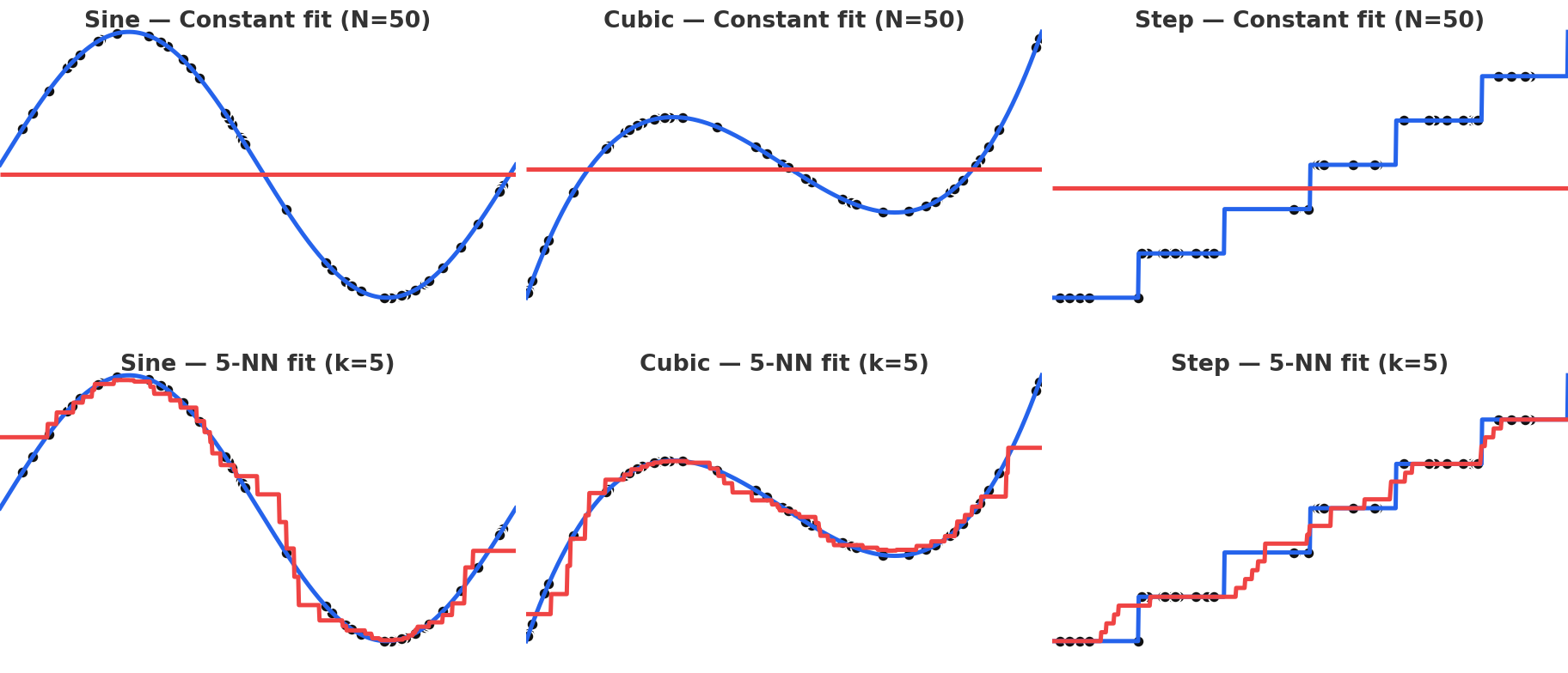Constant regression does significantly worse than a naive local KNN.

This motivates us to modify our model slightly, and instead assume our model is locally constant under some weighting scheme. We will employ some kernel $K$ to upweight datapoints close to the queried input and downweight far away datapoints, making our approach akin to smoothing. We will now solve the kernel-weighted least squares problem.

$\hat{\beta}_0 = \operatorname{arg\,min}_\beta \sum_{i=1}^{n} K_h(x_i, x_0)(y_i - \beta)^2$

The kernel weight is defined as $K_h(x_i, x_0) = K\left(\frac{\|x_i - x_0\|}{h}\right), h>0$ for some kernel function $K$. ²

Minimizing with respect to $\beta$ gives

The RHS of the above equation is referred to as the Nadaraya-Watson (NW) estimator[8][9]. The NW estimator enjoys a rich history in econometrics, statistical modeling, and nonparametric regression theory.

The most common choice of kernel is the Gaussian kernel

$K(u)=e^{-u^2/2} \implies K_h(x_i, x_0)=\exp\left(-\frac{\|x_i - x_0\|^2}{2h^2}\right)$

which has the virtue of being isotropic, continuous, and simple.

Now we make the connection to attention explicit by changing our notation. Let us denote our input vectors as keys $k$ and our response vectors as values $v$. We want to sample our regression problem at a query point $q$, also a vector living in key space.

To connect with modern attention mechanisms, we make two additional assumptions. First, we employ QK-norm, whereby the queries and keys are normalized to unit norm. Second, we define our kernel bandwidth as the square-root-temperature $h=\sqrt{\tau}$.

With these substitutions, our kernel becomes:

Plugging this into the NW estimator, we obtain a familiar culprit.

$\boxed{f(q) = \sum_{i=1}^n \frac{\exp(\frac{qk_i^T}{\tau})}{\sum_{i=1}^n \exp(\frac{qk_i^T}{\tau})} v_i = \mathrm{softmax}(QK^T)V}$

Thus, we have shown that attention arises as a simple solution to an even simpler nonparametric kernel regression problem. The beautiful setting from which attention intuitively arises is a fascinating result. Gaussian kernel NW regression has been employed for decades in econometrics and related disciplines - truly nothing in ML is ever "new".

It's all you need!

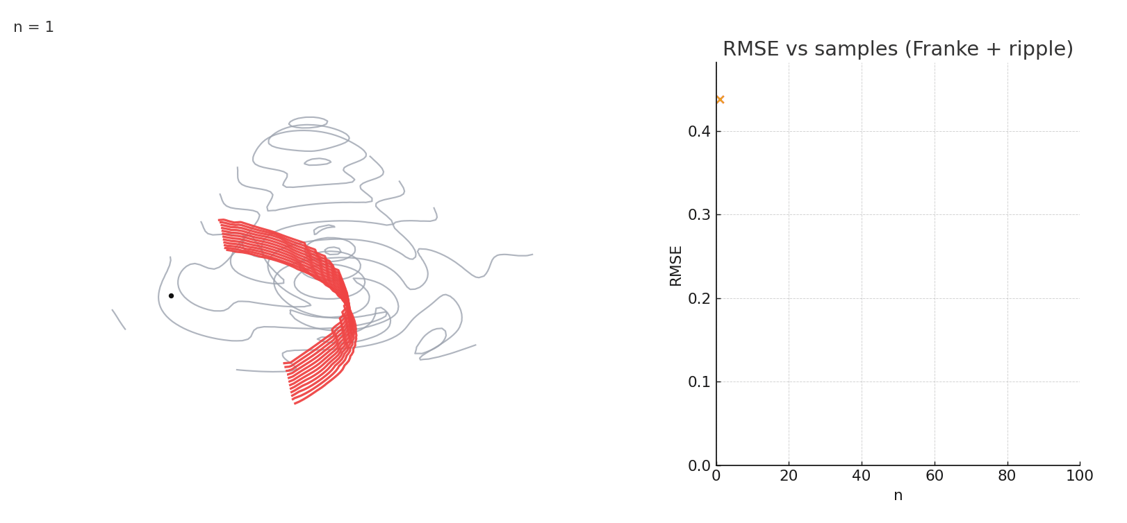
Gaussian NW is quite powerful for fitting arbitrary vector-valued functions, despite being a simple model. Local kernel fits can approximate complex nonlinear functions despite their simple description, with some examples shown below. This flexibility is precisely what makes attention powerful.

Gaussian NW can approximate a wide variety of functional forms, including sinusoidal, polynomial, and even piecewise.

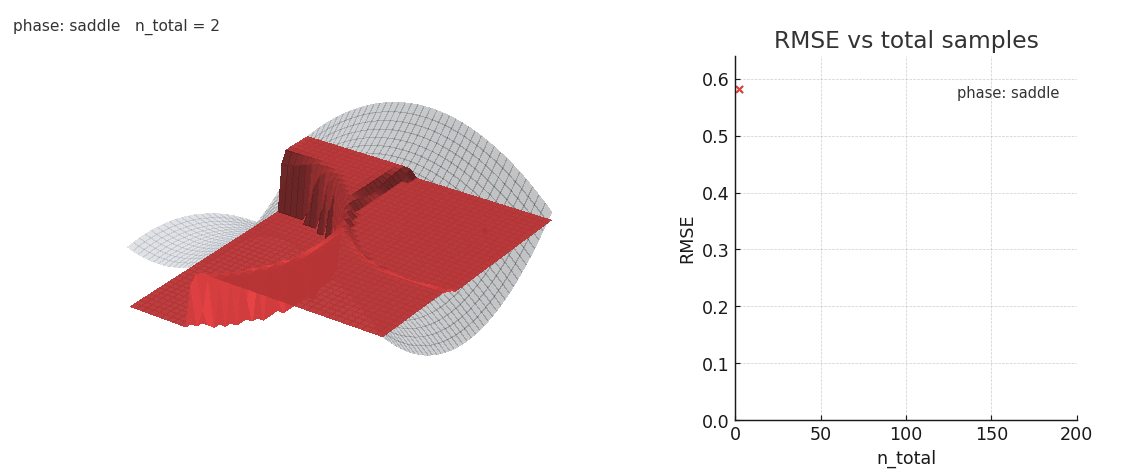
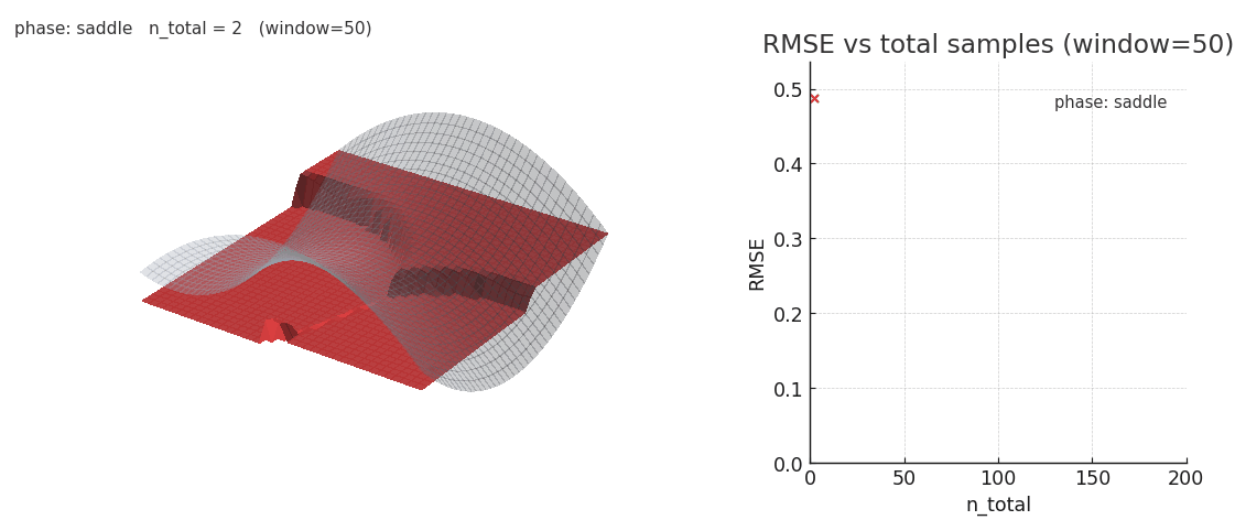
Gaussian NW fitting a complex 3D surface. Error stabilizes after relatively few samples.

However, attention has some difficulty when the distribution of keys/values suddenly shifts. The old regression points are still embedded in the landscape, and the kernel smoothing weights them accordingly.

Sliding window and positional encoding both help to overcome the issue, by offering a natural recency bias. Here's an example of NW under a distribution shift, with and without sliding window:

Gaussian NW fitting a spline surface under in-context distribution shifts. Old keys/values interfere with the fit.

Sliding window gaussian NW is more robust to distribution shifts, at the cost of poorer expressivity.

As seen above, sliding window is worse at fitting the complex surface but is significantly more robust to distribution shifts. It's intriguing to think about the kinds of complex, high-dimensional surfaces transformers could be fitting in-context and how different architectural choices may impact the learned geometry. As we saw in Sparsity is Cool, the emergent geometry of key manifolds is strongly influenced by the choice of sequence mixer and key parametrization.

Kernels on kernels

We may ask what functional forms emerge when we apply other nonparametric kernel smoothers. Another common choice is the Epanechnikov kernel[7], which simplifies as follows under the unit norm assumption.

$K_\tau(q,k)=\max\left(0, 1-\frac{\|q-k\|_2^2}{\tau}\right) = \max\left(0, 1-\frac{2}{\tau}+\frac{2}{\tau}qk^T\right)$

The Epanechnikov kernel is often referred to as the optimal kernel in kernel density estimation (KDE) theory because it is proven to be asymptotically MSE-optimal among second-order kernels. Epanechnikov attention (NW with the Epanechnikov kernel) has a number of favorable properties, including:

• Compact support - a key only contributes if its similarity is above a threshold, allowing higher selectivity. This can reduce interference, such as the GQA noise we identified in Sparsity is Cool. The kernel also naturally introduces sparsity in the attention map. Furthermore, the compact support reduces the effect of outliers.
• Stable attention logits - by doing away with $\exp$, we alleviate exploding attention logits. We avoid the underflow/overflow problem with exponentials.

We can simplify the kernel by constraining the domain of the bandwidth. Nonnegativity of the second term requires $1-\frac{\|q-k\|_2^2}{\tau} \geq 0 \Rightarrow \tau \geq 4$. If the temperature is above this threshold, then the Epanechnikov attention is simply:

A linear attention variant! After all, by eliminating the $\max$ we have removed the nonlinearity.

Indeed, if we had instead defined the feature map

$\phi(x) = \begin{bmatrix} \sqrt{1-\frac{2}{\tau}} \\ \sqrt{\frac{2}{\tau}}x \end{bmatrix} \in \mathbb{R}^{1+d_k} \quad\Rightarrow\quad K_\tau(q,k) = \phi(q)^\top \phi(k)$

Then we have the standard linear attention recurrence:

The Epanechnikov feature map is a special first-order case of the polynomial feature map, which was developed and applied in the linear attention literature previously[10][11][12]. Assuming bandwidth constraints, Epanechnikov attention admits a slick linear form with a known feature map.

Takeaways

A broad class of test-time learning algorithms can be expressed as vector-valued regressors on key-value space; the main difference is that the entire regression problem is programmed in-context. The general framework offers for the fruitful cross-pollination of many concepts from elementary regression theory to the development of hardware-aligned sequence mixers.

There is a rich literature on the perspective of test-time learning with in-context learned key-value maps[2]. Test-time learners can be described simply by a choice of loss function, optimizer, and regularization (e.g. here we have the kernel-weighted least squares loss, an analytical solver, and no regularization respectively)[3].

References

- Sun, Yu and Li, Xinhao and Dalal, Karan and Xu, Jiarui and Vikram, Arjun and Zhang, Genghan and Dubois, Yann and Chen, Xinlei and Wang, Xiaolong and Koyejo, Sanmi and Hashimoto, Tatsunori and Guestrin, Carlos (2024).
- Wang, Ke Alexander and Shi, Jiaxin and Fox, Emily B. (2025).
- Behrouz, Ali and Razaviyayn, Meisam and Zhong, Peilin and Mirrokni, Vahab (2025).
- Tsai, Yao-Hung Hubert and Bai, Shaojie and Yamada, Makoto and Morency, Louis-Philippe and Salakhutdinov, Ruslan (2019).
- Choromanski, Krzysztof and Likhosherstov, Valerii and Dohan, David and Song, Xingyou and Gane, Andreea and Sarlós, Tamás and Hawkins, Peter and Davis, Jared and Mohiuddin, Afroz and Kaiser, Lukasz and others (2021).
- Katharopoulos, Angelos and Vyas, Apoorv and Pappas, Nikolaos and Fleuret, François (2020).
- Epanechnikov, V. A. (1969).
- Nadaraya, E. A. (1964).
- Smooth Regression AnalysisWatson, G. S. (1964).
- Arora, Simran and Eyuboglu, Sabri and Zhang, Michael and Timalsina, Aman and Alberti, Silas and Zou, James and Rudra, Atri and Re, Christopher (2024).
- Kacham, Praneeth and Mirrokni, Vahab and Zhong, Peilin (2024).
- Nauen, Tobias Christian and Palacio, Sebastian and Dengel, Andreas (2024).