Introduction

Modern first-order optimizers can let weight matrices drift into poorly conditioned regimes, amplifying gradient noise and forcing conservative step sizes. Muon mitigates this by orthogonalizing updates, but the weights themselves remain unconstrained. Manifold Muon takes the next step by constraining each linear layer to a geometry—e.g., the Stiefel manifold—so singular values of both the update matrix and the weight matrix are controlled by construction.

In this post, we explore whether this strict constraint can be relaxed. We begin by recapping the original manifold Muon optimizer, then derive two variants by selectively relaxing the constraints on the weight matrix's Gram matrix $(W^\top W)$. Finally, we propose a single, unified framework for designing Gram-space optimizers.

We show how this framework can systematically generate a family of related manifolds—including the Stiefel manifold and its simple relaxations—which inherit the same efficient dual solution and fast $\mathrm{msign}$ computation.

(Manifold) Muon Recap

Muon[1][2] orthogonalizes weight updates to keep linear layers well-conditioned. Recently, Jeremy Bernstein and Thinking Machines released an insightful post[3] in which they introduce a version of the Muon optimizer where the weights of the network are constrained to the Stiefel manifold:

Given a gradient matrix $G$, the "manifold Muon" problem solves

where the spectral-norm bound controls update size and the second constraint enforces $A$ to lie in the tangent space

Note in particular that both the Stiefel constraint and the tangent constraint are natural generalizations of the hyperspherical constraint and its tangent constraint.

As a smooth manifold, we have

and one can think of $\text{Stiefel}(m,n)$ as the set of orthonormal $n$-frames in $\mathbb{R}^m$.

As nicely detailed in [4], in order to solve problem (1) one introduces a matrix $\Lambda\in \mathbb{R}^{n\times n}$ and forms the Lagrangian

where the angle brackets denote the Frobenius inner product $\langle X, Y \rangle := \text{Tr}(X^\top Y)$. By a minimax swap and the fact that

where $\mathrm{msign}(M)$ denotes the matrix polar factor: if $M = U \Sigma V^\top$ is an SVD, then $\mathrm{msign}(M) := U V^\top$ (zeros on singular-zero directions)¹. One then shows that (1) admits the dual problem²:

where the nuclear norm is the sum of the singular values. This problem is then solved by gradient ascent, where a subgradient³ of this dual objective is then given by

where $Z := \text{msign}\big(G + W(\Lambda + \Lambda^\top)\big)$.

A couple of remarks about this derivation:

• Note that although we introduce a full matrix of Lagrange multipliers $\Lambda\in \mathbb{R}^{n\times n}$, in fact only $\text{sym}(\Lambda) = (\Lambda+\Lambda^\top)/2$ actually mattered, so it would have been sufficient to take $\Lambda$ to be symmetric.
• When formulating the manifold Muon problem, there are two size constraints: an explicit size constraint on the size of the update matrix $A$, and a kind of implicit constraint on the weight matrix $W$ (namely that it has unit condition number).

In the next section, we will obtain a different manifold Muon-style optimization problem (though the process of solving it will be remarkably similar to the above). To do so, we will relax the unit condition number requirement.

Manifold Muon in Gram Matrix Space

The Stiefel constraint $W^TW = I$ is in fact just one constraint that one can put on the Gram matrix of a collection of vectors. Let $w_1,\ldots, w_n$ be vectors in $\mathbb{R}^m$ arranged as columns of $W$. The Gram matrix is then

The Gram matrix $\text{Gram}(W)$ encodes the geometry of the column vectors of $W$. Its entries tell us everything about their lengths and the angles between them:

• The diagonal entries ($w_i^\top w_i$) are the squared lengths of each column vector.
• The off-diagonal entries ($w_i^\top w_j$) are the dot products between different columns, measuring their orthogonality.

Using this view, we can equivalently define the Stiefel manifold as (ordered) collections of $n$ vectors in $\mathbb{R}^m$ whose Gram matrix is the $n\times n$ identity matrix.

With this view in mind, we introduce two relaxations of the Stiefel constraint, each obtained by relaxing one aspect of the identity requirement $W^TW = I$:

• Diagonal Gram: Require off-diagonal entries to vanish (orthogonality), but allow diagonal entries to vary (non-unit norms).
• Oblique: Require diagonal entries to equal 1 (unit norms), but allow non-zero off-diagonal entries (non-orthogonality).

Diagonal Gram Manifold Muon

We first consider allowing the Gram matrix $W^\top W$ to be an arbitrary diagonal matrix. Define⁴

Strict positivity of the $\lambda_i$ is needed for $\text{DGram}(m,n)$ to possess the structure of a smooth manifold. In fact, we have an explicit diffeomorphism

Moreover, as

we obtain

so we gain $n$ additional degrees of freedom relative to $\text{Stiefel}(m,n)$.

One can then show that the tangent space at $W$ is

where $\text{Off}(\cdot)$ is the operator that projects to the off-diagonal part of a matrix. In other words, $A^\top W + W^\top A$ must be diagonal.

For gradient $G$ and Lagrange multiplier $\Lambda$, the analogous Lagrangian is then

Note by self-adjointness of the $\text{Off}(\cdot)$ operator, it actually suffices to only consider $\Lambda$ symmetric with zero diagonal.

As in the Stiefel case, one then proceeds by solving the analogous dual formulation

and obtains the following subgradient

Note the similarity in form to the original manifold Muon solution.

Oblique Gram Manifold Muon

Alternatively, we relax the orthogonality requirement while maintaining unit norms. Define

where "oblique" comes from the fact that columns have unit norm but can be mutually oblique (not orthogonal).

In fact, $\text{Oblique}(m,n)$ is diffeomorphic to $(S^{m-1})^n$ by simply mapping each column to a point in $S^{m-1}$, and hence the manifold has dimension $(m-1)n$. In this case, the tangent space is given by

The corresponding Lagrangian is then

The dual problem takes the same form:

and we obtain the subgradient

A Unifying Theme

In fact each of the three examples above are really instances of the following more general setup.

Let $\text{Sym}_n$ denote the space of $n\times n$ symmetric matrices, let

be a self-adjoint linear projector (i.e., $P^2=P$ and $P^\top=P$), and let $\mathcal{C}\subseteq\text{Sym}_n$ be some class of symmetric matrices.

Given $W\in\mathbb{R}^{m\times n}$, it follows that $\text{Gram}(W)$ lies in $\text{Sym}_n$, and $P(\text{Gram}(W))$ lies in $\text{Sym}_n$.

Then each of the optimization problems above is a special case of the following family of manifolds:

Some observations:

• It is sufficient to consider $P$ to have domain $\text{Sym}_n$ since we could otherwise just precompose with the $\text{sym}$ map.
• For any symmetric $X$ and $n\times n$ matrix $M$, we have $\langle M, X\rangle=\langle\text{sym}(M), X\rangle$ since $\langle\text{skew}(M), X\rangle=0$ for any $M$.

Moreover, each of the components of the above problem have a completely general form⁵:

Tangent space:

Lagrangian:

Dual problem:

Subgradient:

The derivation shows that for any self-adjoint projector $P$, the inner minimization over the spectral-norm ball always yields the same nuclear-norm dual with subgradient $Z = \mathrm{msign}(\cdot)$ (the polar factor), so the exact same Newton–Schulz/Polar-Express routine applies—there is no new solver to invent for each choice of $P$.

For example, the three instances above correspond to specifying $(P,\mathcal{C})$ as follows:

• Stiefel: $P=\mathrm{Id}$, $\mathcal{C}=\lbrace I\rbrace$.
• Diagonal-Gram: $P=\text{Off}$, $\mathcal{C}=\lbrace 0\rbrace$.
• Oblique: $P=\text{Diag}$, $\mathcal{C}=\lbrace I\rbrace$.

In particular, we would offer that it may be easier to search for the ideal constraint manifold by instead contemplating what the correct $\mathcal{M}_{P,\mathcal{C}}$ set is.

Results

We follow the experiment from the modular manifolds post[3]. We compare four optimizers—Adam[5], Stiefel–Muon, DGram–Muon, and Oblique–Muon—sweeping learning rates over $\{$1e-3, 3e-3, 1e-2, 3e-2, 1e-1, 3e-1, 1e1, 1e2$\}$.

The figures below summarize train/test accuracy and show the singular-value spectra of the best run per method.

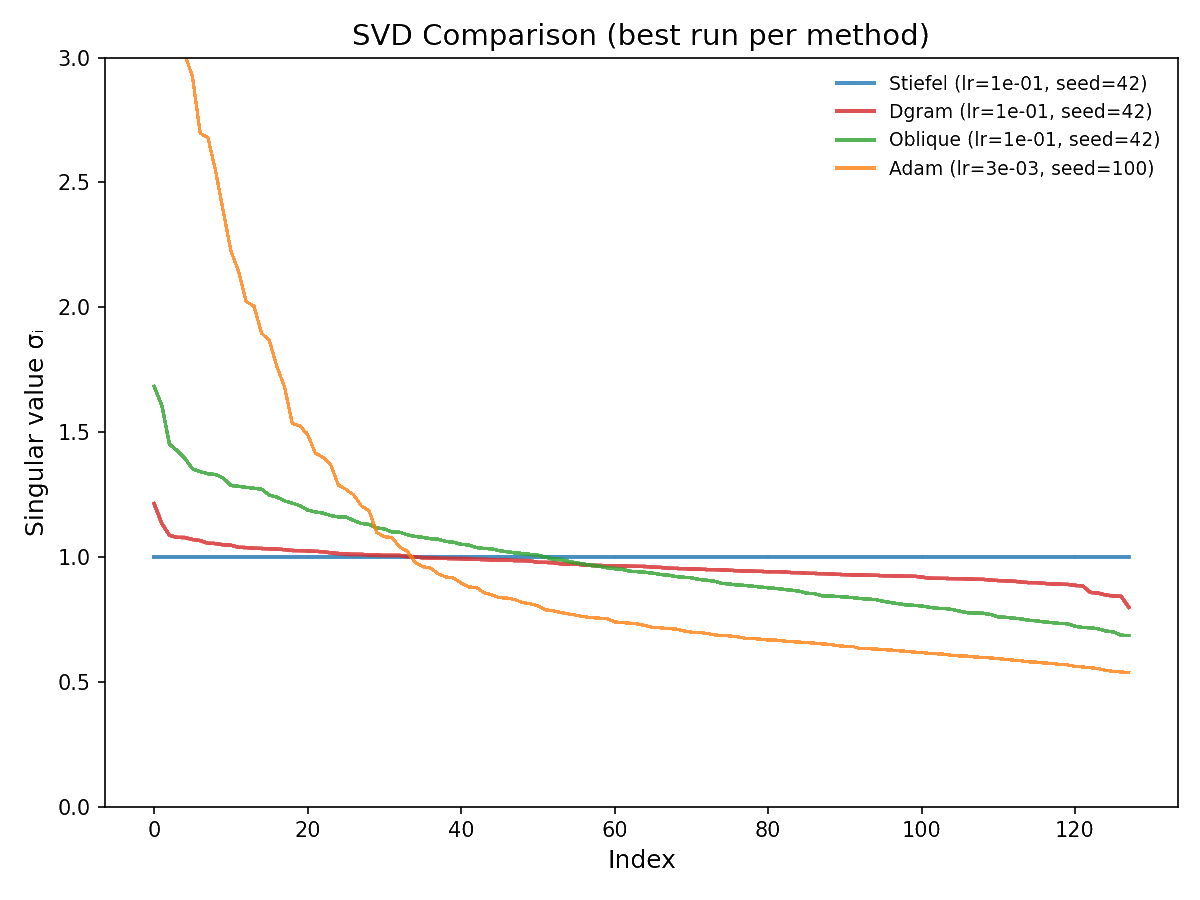Figure 1: SVD statistics across optimizers.

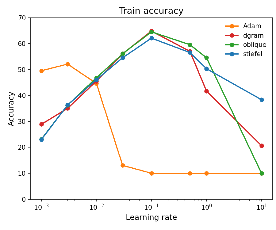Figure 2: Train accuracy across learning rates.

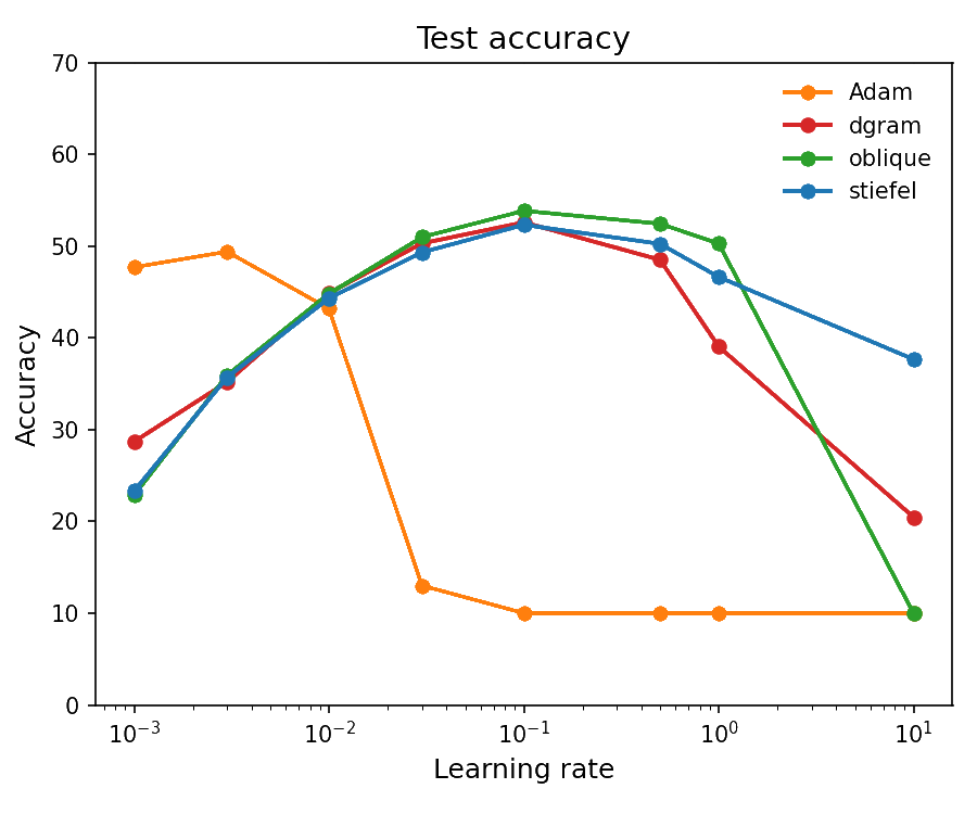Figure 3: Test accuracy across learning rates.

The results reveal an interesting spectrum of conditioning behavior. As expected, Stiefel–Muon maintains condition number 1 by construction. The DGram and Oblique variants exhibit more spread in their singular value distributions, yet still maintain substantially better conditioning than Adam.

It would be very interesting to see if this result scales in any way. That is, it is not obvious to us that one always wants all of the singular values of a weight matrix $W$ to be 1, as is the case for the Stiefel manifold. Adam likely induces far too much variance in the singular value distribution, but allowing slightly more "wiggle room" centered about 1 seems plausible—it could give the model a bit more freedom to privilege certain directions while still maintaining good conditioning. For instance, one could even have a "weight decay"-like term that penalizes deviation from 1.

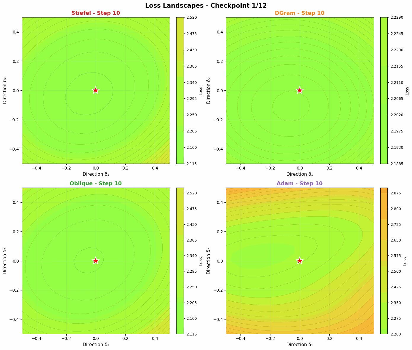
Probing the loss landscape of our MLP over time through random projections reveals a similar intuition. Unlike Adam, DGram and Oblique seem to find smoother, more stable valleys in the loss landscape. Compared with the more constrained Stiefel muon, they then descend faster into the minima. Slightly weakening the orthonormality constraint offers a strong balance of regularization (to find flatter basins) and power (to converge quickly when a basin is found).

Takeaways

Optimizer design involves two complementary choices: selecting the right geometry for gradient descent (via an appropriate norm), and choosing the right manifold to constrain weights to.

We showed that the Stiefel Muon optimization problem extends to a broader family of manifolds $\mathcal{M}_{P,\mathcal{C}}$ parameterized by self-adjoint projectors $P$ on the space of symmetric matrices and constraint sets $\mathcal{C}$. The solution method—passing to a dual problem involving the nuclear norm—remains structurally identical across this family.

This suggests that manifold selection might be more naturally approached through Gram-space design: rather than directly specifying geometric constraints on $W$, we can work in the space of Gram matrices and choose which geometric invariants to constrain via $P$ and $\mathcal{C}$.

Acknowledgments

In addition to the post this work is based on, there are some other very[6] nice [7] posts on the topic of manifold-constrained optimizers.

References

- Bernstein, Jeremy (2024).
- Jordan, Keller et al. (2024).
- Bernstein, Jeremy (2025).
- Kingma, Diederik P. and Ba, Jimmy (2014).
- Cesista, Franz Louis (2025).
- Su, Jianlin (2025).
Footnotes
-
Equivalently, is the polar factor in ; with SVD it reduces to (with zeros on null singular spaces). In practice we compute efficiently via Newton–Schulz or Polar-Express iterations, avoiding an explicit SVD. ↩
For the full details on the argument, see [4]. ↩
One must use subgradients here because the nuclear norm is convex but not everywhere differentiable ↩
In practice you may want bounds on the diagonal entries, e.g. with , to avoid degeneracy and runaway scaling. ↩
One also has a closed form for retraction maps (which depend on ) for this general setup. ↩